What is Agentforce Revenue Management?
What is Agentforce Revenue Management? April 26, 2026 Posted by: SFDCGYM Category: Revenue Cloud , No Comments Home For years,...
Read More →


Data Spaces offer organizations the ability to fine-tune data access and maintain security boundaries. Key uses include:
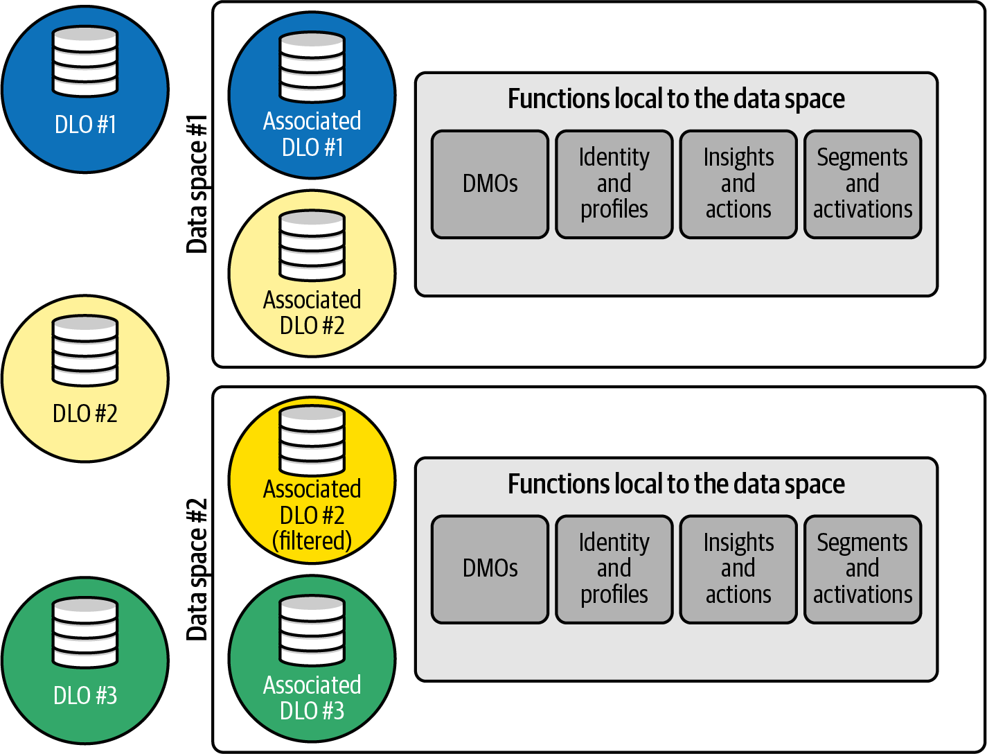
For administrators dealing with large and complex databases, Data Spaces provide a crucial mechanism for maintaining order and access control within the Data Cloud framework.
Creating a Data Space is straightforward when done via your Data Cloud platform. Follow these steps:
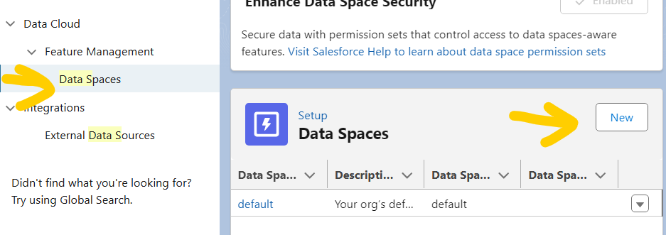
Once the Data Space is created, you can start organizing your data within its logical boundaries.
Once your Data Space is set up, the next crucial step is to control who can access it. Access management is driven by Permission Sets within the Data Cloud. Here’s how you can assign permissions:

With Permission Sets, you can ensure that only authorized personnel can access or manage specific Data Spaces in your Data Cloud environment.